彩笔运维勇闯机器学习--逻辑回归

前言

从本节开始，我们的机器学习之旅进入了下一个篇章。之前讨论的是回归算法，回归算法主要用于预测数据。而本节讨论的是分类问题，简而言之就是按照规则将数据分类

而要讨论的逻辑回归，虽然名字叫做回归，它要解决的是分类问题

开始探索

scikit-learn

还是老规矩，先来个例子，再讨论原理

假设以下场景：一位老哥想要测试他老婆对于抽烟忍耐度，他进行了以下测试

将以上情形带入模型

from sklearn.linear_model import LogisticRegressionimport numpy as npX = np.array([6, 18, 14, 13, 5, 10, 8]).reshape(-1, 1)y = np.array([0, 1, 1, 1, 0, 1, 0])model = LogisticRegression()model.fit(X, y)print(f"系数： {model.coef_[0][0]:.4f}")print(f"截距： {model.intercept_[0]:.4f}")decision_boundary = -model.intercept_[0] / model.coef_[0][0]print(f"决策边界： {decision_boundary:.2f}")

脚本！启动：

报告解读

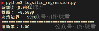
单特征影响结果，这明显是一个线性模型，所以出现了熟悉的系数与截距，还有一个新的参数：决策边界，这意味着9.1就是分类阈值，>=9.1的结果分类为1，<9.1为0

带入到情景当中，每天9根烟以上，要被老婆打，否则不打

深入理解逻辑回归

与线性回归比较

那位大哥说了，怎么和线性回归这么相似，但是最后又有一点不同

• 逻辑回归是将线性回归的输出，再通过函数映射成概率值(0~1之间)，再进行分类
• 线性回归的损失函数是MSE，而逻辑回归的损失函数则是平均交叉熵
• 线性回归的回归系数算法可以用最小二乘法或者梯度算法（之前没有介绍过），逻辑回归只能用梯度算法
• 还有很多不同，包括但不限：评估模型、使用场景、目标函数等都不一样

总之，逻辑回归虽然也有“回归”2字，但是主要还是更适合分类问题

数学模型

逻辑回归通过将线性回归的输出映射到概率值（0到1之间），利用Sigmoid函数（或称逻辑函数）实现分类

w 是权重向量，b是偏置项，X 是输入特征向量

通过该函数，把线性方程的值域从((-infty,+infty))，修改为概率的值域([0,1])

损失函数

与线性回归的mse不同，逻辑回归使用的损失函数为平均交叉熵

from sklearn.metrics import log_lossy_proba = model.predict_proba(X)[:, 1]loss_sklearn = log_loss(y, y_proba)print('=='*20)print(f"损失函数（Log Loss）: {loss_sklearn:.4f}")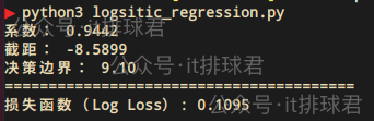

• 值接近0，预测概率接近真实
• 值越大，预测概率错误或不确定
• 趋于(+infty)，极端错误（比如预测为1但是0）

模型评估

• 准确率：顾名思义，分类的准确率

  from sklearn.metrics import accuracy_scorey_pred = model.predict(X)accuracy = accuracy_score(y, y_pred)print('=='*20)print(f"准确率：{accuracy:.2f}")

  

• 混淆矩阵：对于一个二分类（二元问题，最后的结果可以用0、1来分类）问题，混淆矩阵是一个 2×2 的矩阵，包含以下四个关键指标

  • 真正例（TP）：模型正确预测为正例的样本数。比如例子中的“挨打”
  • 假负例（FN）：模型错误预测为正例的样本数（误报）。例子中错误判断为“挨打”
  • 假正例（FP）：模型错误预测为负例的样本数（漏报）。例子中错误判断为“没有挨打”
  • 真负例（TN）：模型正确预测为负例的样本数。比如例子中的“没有挨打”

  [[3 1]  # TN=3, FP=1 [1 3]] # FN=1, TP=3

  from sklearn.metrics import confusion_matrixprint('=='*20)print('混淆矩阵：')y_pred = model.predict(X)cm = confusion_matrix(y, y_pred)print(cm)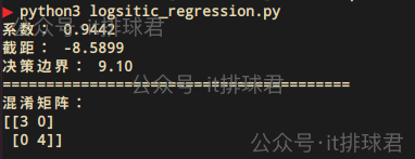

  

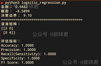
  从混淆矩阵中产生了一系列评估指标：

  • 准确率（accuracy）：模型预测正确的比例 (frac{TP+TN}{TP+TN+FP+FN})
  • 精确率（precision）：预测为正例的样本中，真实为正例的比例 (frac{TP}{TP+FP})
  • 召回率（recall）：真实为正例的样本中，被正确预测的比例 (frac{TP}{TP+FN})
  • 特异度（specificity）：真实为负例的样本中，被正确预测的比例 (frac{TN}{TN+FP})
  • F1分数：精确率和召回率的调和平均数 (2⋅frac{精确率times召回率}{精确率+召回率})

  

  或者直接使用classification_report：

  from sklearn.metrics import classification_reportprint('=='*20)y_pred = model.predict(X)print("Logistic Regression 分类报告:n", classification_report(y, y_pred))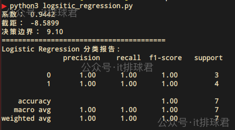

  

• ROC-AUC

  • ROC（受试者工作特征）曲线与AUC（曲线下面积），在类别不平衡的场景中广泛使用。所谓类别不平衡，就是在样本中类别数量差异较大的情况，比如在100w日志当中，99.9%都是正常的，只有0.1%的日志是异常的

  from sklearn.metrics import roc_curve, roc_auc_scorey_proba = model.predict_proba(X)[:, 1]auc_score = roc_auc_score(y, y_proba)print('=='*20)print(f"AUC = {auc_score:.4f}")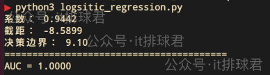

  

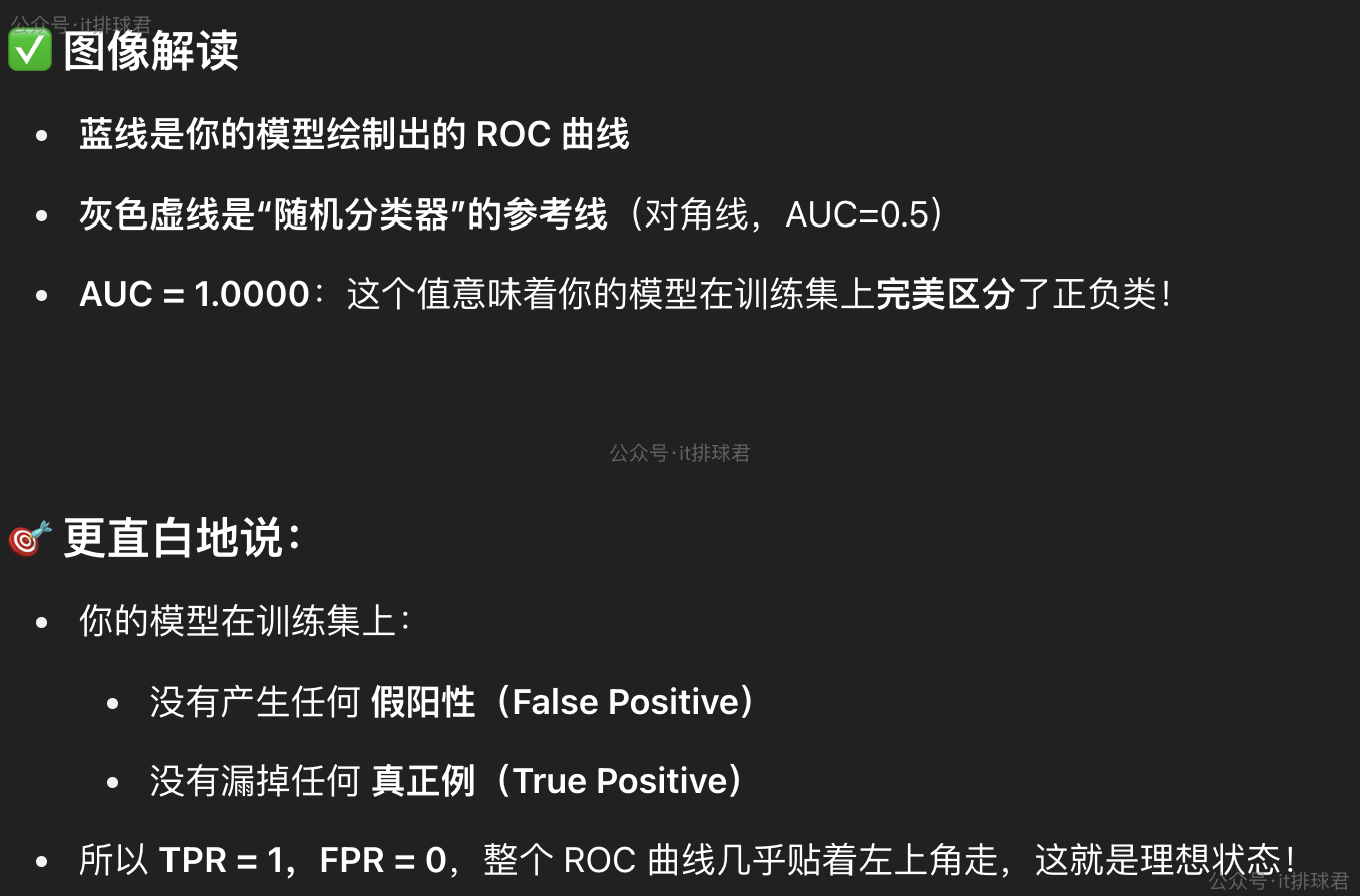
  • AUC越接近1，表示分类模型泛化能力越好，如果在0.5左右，代表着跟猜的一样差

  import matplotlib.pyplot as pltfpr, tpr, thresholds = roc_curve(y, y_proba)plt.figure(figsize=(6, 5))plt.plot(fpr, tpr, color='blue', label=f'ROC curve (AUC = {auc_score:.4f})')plt.plot([0, 1], [0, 1], color='gray', linestyle='--')plt.xlabel('False Positive Rate')plt.ylabel('True Positive Rate')plt.title('ROC Curve')plt.legend()plt.grid(True)plt.tight_layout()plt.show()

  

  直接丢gpt看下吧

  

多特征下的逻辑回归

决策边界

先来讨论一下决策边界，决策边界是先推导出回归系数与截距之后，再带入模型

如果是单特征：

取分类阈值为0.5，为什么要取0.5，大部分情况，二分类中0和1的可能性是均等的，通常任务>0.5为1，反之<0.5则为0。但是遇到所谓的分类不平衡的情况，就要变化了，这个后面再讨论，这里先姑且取0.5

可以看到单特征的决策边界是一个点，这就非常容易区分0和1了

如果是2个特征：

同理(hat{y}=0.5)

可以看到2个特征的决策边界是y=x的直线

同理3个特征是一个面，>3个特征就已经不能画出来了

2个特征

继续刚才的问题，比如除了抽烟被打，再加上喝酒，2个特征

from sklearn.linear_model import LogisticRegressionfrom sklearn.metrics import classification_reportimport numpy as npX = np.array([    [6,8],    [18,1],    [14,2],    [13,4],    [5,3],    [10,3],    [8,0],])y = np.array([1, 0, 0, 1, 0, 1, 1])model = LogisticRegression()model.fit(X, y)coef = model.coef_[0]intercept = model.intercept_[0]print(f"系数： {coef}")print(f"截距： {intercept}")

决策边界：$$ y=frac{0.127x-0.94}{0.26} $$

import matplotlib.pyplot as pltx_vals = np.linspace(X[:, 0].min() - 1, X[:, 0].max() + 1, 100)decision_boundary = -(coef[0] * x_vals + intercept) / coef[1]plt.figure(figsize=(8, 6))colors = ['red' if label == 0 else 'blue' for label in y]plt.scatter(X[:, 0], X[:, 1], c=colors, s=80, edgecolor='k')plt.plot(x_vals, decision_boundary, 'k--', label='Decision Boundary')plt.legend()plt.grid(True)plt.tight_layout()plt.show()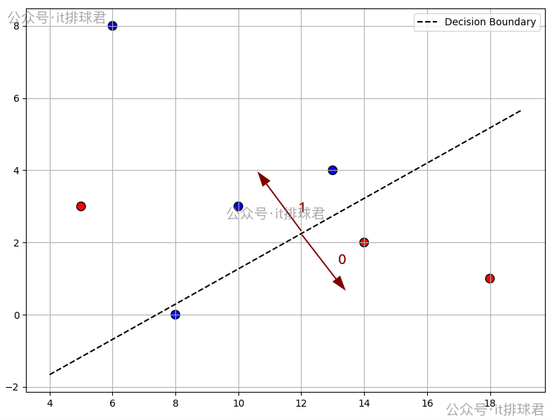

在边界以上的是1，边界以下的0

类别不平衡

比如以下代码，1000个样本中，只有14个1，986个0，属于严重的类别不平衡

from sklearn.linear_model import LogisticRegressionfrom sklearn.datasets import make_classificationfrom sklearn.metrics import classification_reportfrom sklearn.model_selection import train_test_splitX, y = make_classification(n_samples=1000, n_features=5,                          weights=[0.99], flip_y=0.01,                          class_sep=0.5, random_state=0)X_train, X_test, y_train, y_test = train_test_split(X, y, test_size=0.3)model = LogisticRegression()model.fit(X_train, y_train)y_pred = model.predict(X_test)c_report = classification_report(y_test, y_pred, zero_division=0)print("Logistic Regression 分类报告:n", c_report)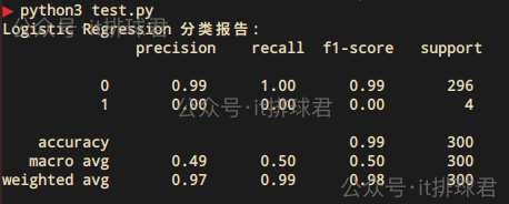

• precision：模型在识别少数类1上完全失败，虽然多数类0的准确率是99%，但是毫无意义，从未正确预测为1
• recall：所有真正为0的样本都被找到了（100%）；一个1类都没找到
• f1-score：类别1的 F1 是 0，说明模型对少数类的预测能力完全崩溃
• support：类别0有 296 个样本，类别1只有 4 个样本
• accuracy：0.99，模型总共预测对了 296 个，错了 4 个
• macro avg：每个类的指标的“简单平均”，不考虑样本数权重
• weighted avg：各类指标的“加权平均”，考虑样本量

有位彦祖说了，你这分类只分了1次训练集和测试集，如果带上交叉验证，多分几次类，让其更有机会学习到少数类，情况能不能有所改善？

from sklearn.model_selection import cross_val_predictcv = StratifiedKFold(n_splits=5, shuffle=True, random_state=0)y_pred = cross_val_predict(model, X, y, cv=cv)c_report = classification_report(y, y_pred, zero_division=0)print("Logistic Regression（交叉验证）分类报告:n", c_report)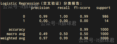

情况并没有好转，模型依然无法区分少数类

权重调整

model = LogisticRegression(class_weight='balanced')model.fit(X_train, y_train)y_pred = model.predict(X_test)c_report = classification_report(y_test, y_pred, zero_division=0)print("Logistic Regression 加权 分类报告:n", c_report)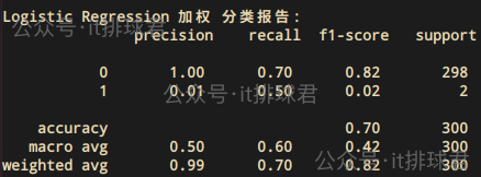

情况有所好转

• 1的recall从0-->0.5，2 个正类样本中至少预测中了 1 个
• 1的Precision从0-->0.01，模型预测为正类的样本大多数是错的，这是 class_weight 造成的：宁愿错也要猜一猜正类
• 0的recall从1-->0.7，同样是class_weight造成的，把一部分原本是负类的样本错判为正类了
• accuracy从99%-->70%，模型开始尝试预测少数类，虽然整体正确率下降，但变得更愿意去预测少数类了

过采样

增加少数类样本，复制或生成新样本，通过 SMOTE（Synthetic Minority Over-sampling Technique）进行过采样

from imblearn.over_sampling import SMOTEfrom imblearn.pipeline import Pipelinefrom sklearn.model_selection import cross_val_predictmodel = Pipeline([    ('smote', SMOTE(random_state=0)),    ('logreg', LogisticRegression(solver='lbfgs', max_iter=1000))])cv = StratifiedKFold(n_splits=5, shuffle=True, random_state=0)y_pred = cross_val_predict(model, X, y, cv=cv)print("SMOTE + LogisticRegression 分类报告:n")print(classification_report(y, y_pred, zero_division=0))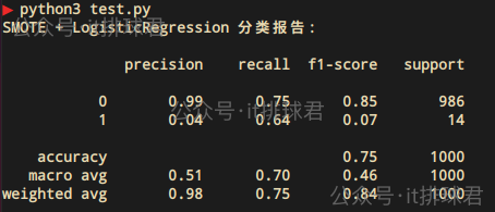

• recall提升到了0.64，模型识别了少数类的概率提升了
• Precision=0.04，精确率依旧不佳
• accuracy=0.75，由于少数类的识别概率提升，所以整体的准确率有所提升

欠采样

减少多数类样本（随机删除或聚类），通过RandomUnderSampler进行欠采样

from imblearn.under_sampling import RandomUnderSamplerfrom imblearn.pipeline import Pipelinefrom sklearn.model_selection import cross_val_predictpipeline = Pipeline([    ('undersample', RandomUnderSampler(random_state=0)),    ('logreg', LogisticRegression(solver='lbfgs', max_iter=1000))])cv = StratifiedKFold(n_splits=5, shuffle=True, random_state=0)y_pred = cross_val_predict(pipeline, X, y, cv=cv)print("欠采样 + LogisticRegression 分类报告：n")print(classification_report(y, y_pred, zero_division=0))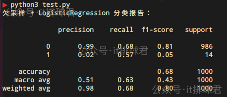

与过采样大同小异，效果还不如过采样

正则化

lasso与Ridge在这里依然可以使用

from imblearn.pipeline import Pipelinefrom sklearn.model_selection import cross_val_predictpipeline = Pipeline([    ('smote', SMOTE(random_state=0)),    ('lasso', LogisticRegression(penalty='l1', solver='liblinear', max_iter=1000, random_state=0))])cv = StratifiedKFold(n_splits=5, shuffle=True, random_state=0)y_pred = cross_val_predict(pipeline, X, y, cv=cv)print("SMOTE + Lasso Logistic Regression（L1）分类报告：n")print(classification_report(y, y_pred, zero_division=0))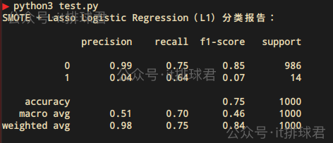

代价敏感学习

这其实也是其中调整的一种，只不过针对于class_weight这个超参数，进行了更精细化得调整

from imblearn.pipeline import Pipelinefrom sklearn.model_selection import cross_val_predictpipeline = Pipeline([    ('smote', SMOTE(random_state=0)),    ('lasso', LogisticRegression(class_weight={0: 1, 1: 50}))])cv = StratifiedKFold(n_splits=5, shuffle=True, random_state=0)y_pred = cross_val_predict(pipeline, X, y, cv=cv)print("class_weight {0:1, 1:50} 分类报告：n")print(classification_report(y, y_pred, zero_division=0))

class_weight={0: 1, 1: 50} 的含义：

• 类别 0（多数类）的权重为 1（标准惩罚）
• 类别 1（少数类）的权重为 50（错误预测时惩罚更严重）

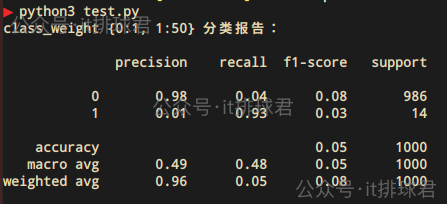
这是一种牺牲准确率为代价，尽量不要漏掉任何一个少数类，所以表现就是少数类1的precision很低，但是recall是非常高的。这就是所谓的宁可错杀一千，也绝不放过一个

小结

在逻辑回归中，针对类别不平衡的问题，往往有两种决策

• 一种是宁可误报，也不能漏报。先把少数类找出来，再对少数类进行进一步的校验。比如预测入侵筛查、代码漏洞检测等
• 另外一种则是需要更关注多数类，有少数类被误报，也是可以接受。比如垃圾邮件分类、推荐系统的准确率等

联系我

• 联系我，做深入的交流
  

至此，本文结束
在下才疏学浅，有撒汤漏水的，请各位不吝赐教...